Pierre-Yves Gousenbourger, Applied Mathematics

Bidimensional interpolation with Bézier spline

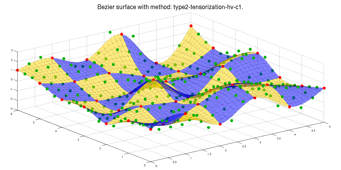
We are given a set of data points in the Euclidean space associated with two timestamps (m,n) organised on a regular grid. These timestamps give the order in which points must be interpolated. In this problem, for visualization convenience and without loss of generality, the (x,y) value of the data points correspond to the regular grid (m,n) and the z-value is randomly chosen. The points are organized in a 2D-cell corresponding to the order of interpolation.

From these data points, the goal here is to draw a 2d-Bézier spline interpolating those in a $C^1$ way. For this, you can use our code here, general for manifolds. The possible manifolds are the Euclidean space, the sphere and the special orthogonal group SO(3).

Download the code.

Show/hide the code tutorial.

The code

Here is the code for interpolating data with a 2d-Bézier spline.

% Some random data points.
m = 6; n = 7;
data = cell(m,n);
for i=1:m
for j=1:n
  data{i,j} = [i-1,j-1,randn(1)];
end
end

% Some useful information...
manifold = 'euclidean';
set_path
global_variables
geo_functions

% Create the problem structure.
problem  = prepare_structure(data,manifold,10);

% Phase 1: Control points generation.
problem = control_points_simple_generation_2d(problem);

% Phase 2: Reconstruction of the curve.
problem = curve_reconstruction_double_bezier_c1(problem,1); % horizontal-vertical

% Plotting
figure;
draw_bezier_surface(problem);
title(['Bezier surface with method: ',problem.method,'.']);

Okay, let's dig a bit into that...

Data points

As mentionned, the data points must be stored in a 2d-cell. Let's construct a random set of data points where the (x,y)-values correspond to (m,n) and the z-value is random.

Hint: You may also call data_points_2d(manifold,type) to create some predefined test sets.

m = 6; n = 7;
data = cell(m,n);
for i=1:m
for j=1:n
  data{i,j} = [i-1,j-1,randn(1)];
end
end

Problem structure preparation

The system is based on a structure called successively by different subfunctions in matlab. Each subfunction will use elements of differential geometry (the exponential, the logarithm, the distance, etc.). This is why this preparation step is crucial in order to inform the computer on the paths needed (the script set_path depends on the manifold) and on the elements of differential geometry available for the code (global_variables and geo_functions depend on the manifold).

manifold = 'euclidean';

% define the paths where the manifold-tools are stored
set_path
% define the global variables, i.e. the elements of differential geometry.
global_variables
geo_functions

Create the problem structure.

% the structure stored the name of the manifold, the data points and the discretization of the surface when reconstructed.
problem  = prepare_structure(data,manifold,10);

The structure should look like

problem = 				
interp: {6x7 cell}
type: ''
manifold: 'euclidean'
   n: 6
   m: 7
dim1: 1
dim2: 3
   d: []
   t: 10
nint: 0

Bézier spline optimization and reconstruction

The interpolation problem works in two steps:

find the control points leading the Bézier curve
reconstruct the actual spline.

Phase 1: Control points generation

The subfunction takes the structure as entry and will update it by adding the computed control points.

problem = control_points_simple_generation_2d(problem);

There exist different methods to compute the control points:

control_points_generation(problem): By an exact technique minimizing the Euclidean acceleration of the path. Warning, this technique is costly in time when the log and exp are not trivial. The technique is documented in the technical report of 2015.
control_points_simple_generation_2d(problem) With an efficient but not perfect algorithm based on the B-spline representation of curves generalized to surfaces. This technique is documented in ESANN2016
control_points_double_tensorization(problem) With the same efficient algorithm but applied to 1D curves horizontally and then vertically. The technique is also documented in ESANN2016

In the Euclidean space, all these techniques are identical.

Phase 2: Reconstruction of the curve

Here also, the subfunction takes the structure as entry and will update it by adding the computed spline. If the structure does not contain the control points, the reconstruction is not possible.

problem = curve_reconstruction_double_bezier_c1(problem,1); % horizontal-vertical

There also exist different techniques to reconstruct the Bézier spline. The following ones return a C^1 surface. They are documented in technical report of 2015.

curve_reconstruction_mean_all_c1(problem) uses the altered defintion of Bezier surfaces based on averaging of all control points of the patch.
curve_reconstruction_double_bezier_c1(problem,k) uses the altered definition of Bezier curves horizontal-vertical (k=1) or vertical-horizontal (k=2) depending on the argument.

The two following ones return a C^0 surface and their limits are also discussed in the technical report of 2015.

curve_reconstruction_mean_all(problem) uses the basic definition of Bezier surfaces based on averaging of all the points of the patch.
curve_reconstruction_double_bezier(problem,k) uses the basic definition of Bezier curves horizontal-vertical (1) or vertical-horizontal (2) depending on the argument.

Plotting

We propose a method to plot the solution. The plotting method is chosen based on the manifold and on the paths set at the beginning.

figure;
draw_bezier_surface(problem);
title(['Bezier surface with method: ',problem.method,'.']);

Unidimensional interpolation with hybrid composite Bézier curves

We are given a set of data points in the Euclidean space associated with a timestamp $t_i \in \mathbb{Z}$. We would like to compute a composite Bézier curve that interpolates the data points $d_i$ at time $t_i$. In this problem, we try to interpolate four data points $d_i \in \mathbb{S}^2$, the unit sphere. These points are places such that they represent a triangle.

To fit the curve $\mathfrak{B}(t): [0,3] \to \mathbb{S}^2$, you can use our code here, general for manifolds. The possible manifolds are the Euclidean space, the sphere, the special orthogonal group SO(3),... actually all manifolds you can find in Manopt are operational. It is however mandatory to add manopt to your working path. The zip file hereunder contains an old version of Manopt for consistency. You can download the last version of Manopt here (recommended) : www.manopt.org.

Download the code.

Show/hide the code tutorial.

The code

Here is the code for interpolating data with a hybrid composite Bézier curve on the sphere.

% Add the paths for manopt and for the tools
cd manopt;
addpath(genpath(pwd));
cd ..;
addpath(genpath([pwd,'/tools']));
  
% Some data points on the sphere.
phi     = [pi/3 ; 4*pi/7 ; 4*pi/7 ; pi/3] - 2*pi/12; 
theta   = [pi/2 ; pi/4 ; 3*pi/4 ; pi/2] + 10*pi/12;
x       = cos(theta).*sin(phi); y = sin(theta).*sin(phi); z = cos(phi);
points  = [x y z];
data    = reshape(points',1,3,4);

% Problem parameters
n = size(data,3);
t = linspace(0,n-1,100);

% Structure creation
problem.M = spherefactory(3);
problem.data = data;

% Phase 1: Control points generation.
problem.control = cp_arnould(problem);

% Phase 2: Reconstruction of the curve.
problem = bezier_reconstruction(problem,t);

% Optional: velocity and acceleration computation.
problem.velocity = bezier_velocity(problem,t);
problem.acceleration = bezier_acceleration(problem,t);
  
% Plotting
y = squeeze(problem.curve)'; b = squeeze(problem.control)'; p = squeeze(problem.data)';	
a = problem.acceleration; v = problem.velocity;

[X,Y,Z] = sphere(); 
figure;
subplot(2,2,[1 3]); surf(0.95*X,0.95*Y,0.95*Z,...
    'FaceAlpha',0.7,'EdgeAlpha',1,...
    'FaceColor', [238 197 145]/255);
  hold on;
  plot3(y(:,1),y(:,2),y(:,3),'b','LineWidth',2);
  plot3(b(:,1),b(:,2),b(:,3),'.','Color',[0 0.7 0],'Markersize',30);
  plot3(p(:,1),p(:,2),p(:,3),'.r','Markersize',30);
  title('Bezier spline');
subplot(222); plot(t(2:end-1),v,'-b','LineWidth',2); title('velocity');
subplot(224); plot(t(2:end-1),a,'-b','LineWidth',2); title('acceleration');

Okay, let's dig a bit into that...

Data points

The data points must be stored in a (l,c,n) matrix, where (l,c) is the matrix size of the embedded space. Here, for the sphere, it would be (1,3), as $\mathbb{S}^2$ is embedded in $\mathbb{R}^3$. The points here are draw a triangle on the sphere, and the first and last points coincide.

Hint: You may also call data_points(manifold,type) to create some predefined test sets. Do not forget to add the path to it (addpath([pwd,'/data_points']);).

% Some data points on the sphere.
phi     = [pi/3 ; 4*pi/7 ; 4*pi/7 ; pi/3] - 2*pi/12; 
theta   = [pi/2 ; pi/4 ; 3*pi/4 ; pi/2] + 10*pi/12;
x       = cos(theta).*sin(phi); y = sin(theta).*sin(phi); z = cos(phi);
points  = [x y z];
data    = reshape(points',1,3,4);

Problem structure preparation

The system is based on a structure called successively by different subfunctions in matlab. Each subfunction will use the elements of differential geometry (the exponential, the logarithm, the distance, etc.) extracted from Manopt and stored in that structure. The names of the different elements of the structure will be very important as they are used by the rest of the code later on.

We prepare first the time parameter t to be able, later on, to compute the reconstruction spline. Typically, it is a discretization of the domain (here $t \in [0,3]$).

% Problem parameters
n = size(data,3);
t = linspace(0,n-1,100);

Now, we store the crucial information in a structure.

% Structure creation
problem.M = spherefactory(3);
problem.data = data;

The structure problem is supposed to be at the end composed of the following elements (in this specific problem):

problem = 				
            data: [1×3×4 double]
               M: [1×1 struct]
         control: [1×3×8 double]
           curve: [1×3×100 double]
        velocity: [98×1 double]
    acceleration: [98×1 double]

The data points are stored in the field data, the control points in control, the curve in curve and the manifold in M. It is important to respect these four names. The other names have less importance.

Bézier curve optimization and reconstruction

The interpolation problem works in two steps:

find the control points leading the Bézier curve
reconstruct the actual spline.

Phase 1: Control points generation

The subfunction takes the structure as entry and will return the control points. Store it in the structure for reconstruction.

problem.control = cp_arnould(problem);

There exist different methods to compute the control points:

cp_arnould(problem): technique proposed in the paper Arnould et al. 2015. This technique is recommended.
cp_gousenbourger(problem): suboptimal technique proposed in the paper Gousenbourger et al. 2014, where the velocity vectors must be specified in the beginning of the method. It works but... well, there is better, so why not using it ? ;-).

Phase 2: Reconstruction of the curve

Here also, the subfunction takes the structure as entry and will update it by adding the computed spline. If the structure does not contain the field control, filled with the control points returned by the control points generation method, the reconstruction is not possible.

problem = bezier_reconstruction(problem,t);

The method is a simple De Casteljau algorithm adapted to compute a hybrid composite Bézier curve.

Optional phase: Acceleration and velocity of the curve

Once the curve is reconstructed, we offer a generic code to evaluate the velocity and the acceleration of the curve. Just use the following piece of code:

a = bezier_velocity(problem,t);
v = bezier_acceleration(problem,t);

Be sure that the field curve is available in the structure problem.

The rest is just plotting the curve on a sphere. Try it :-) !

License

The code provided here is copyright and distributed under the terms of the GNU General Public License (GPL) version 3 (or later).

In short, this means that everyone is free to use the provided code, to modify it and to redistribute it on a free basis. However, this code is not in the public domain; it is copyrighted and there are restrictions on its distribution (see the license and the related frequently asked questions). For example, you cannot integrate this version of the code (in full or in parts) in any closed-source software you plan to distribute (commercially or not). Please contact me for more information.

This section was inspired by the very good Gabriel Peyré's Numerical Tours.